Multiple Scatter Correction (MSC) - Part 1

As in previous posts, we are going to follow the Soil spectroscopy training material and we are going to use the reference material provided.

You can find several posts about MSC in: nir-quimiometria.blogspot.com.

You can also read the explanation of the reference material in the Soil spectroscopy training material.

As always we load our data and the packages we need:

library(tidyverse)
library(prospectr)
load("C:/BLOG/Workspaces/NIR Soil Tutorial/post5.RData")

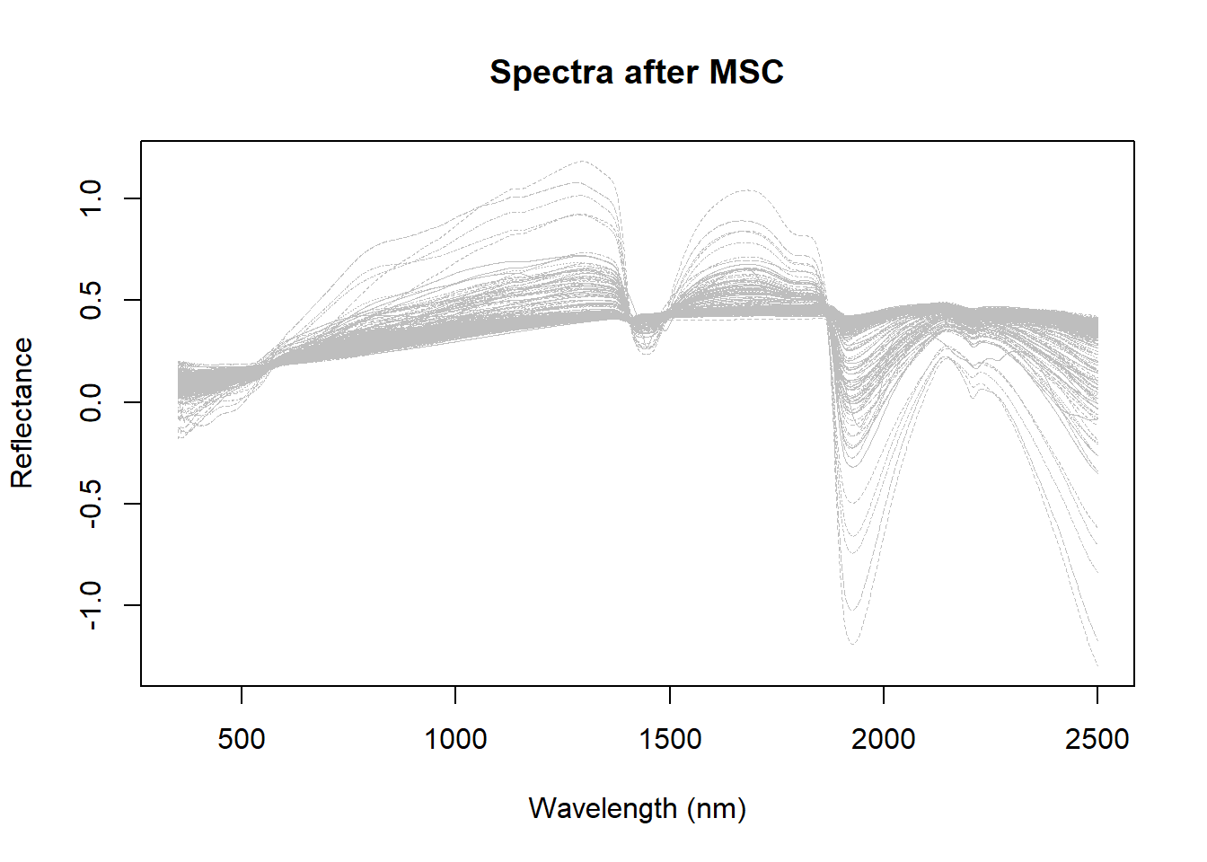
msc_spectra <- msc(dat$spc, ref_spectrum = colMeans(dat$spc))

Let´s use now classical R to see the spectra:

matplot(colnames(dat$spc),
  t(msc_spectra),
  type = "l",
  col = "grey",
  lwd = 0.5,
  xlab = "Wavelength (nm)",
  ylab = "Reflectance",
  main = "Spectra after MSC"
)

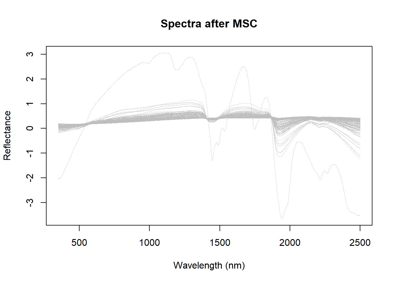
As we can see the scatter effect is minimized, but at the same time we see a sample that is very different from the others. One idea can be to remove this sample and recalculate the MSC.

# Compute the mean reflectance per sample
msc_mean_reflectance <- rowMeans(msc_spectra)

# Get the sample index with the highest mean reflectance
msc_out_sample_index <- which.min(msc_mean_reflectance)

msc_out_sample_index

[1] 102

matplot(colnames(dat$spc),
  t(msc_spectra),
  type = "l",
  col = "grey",
  lwd = 0.5,
  xlab = "Wavelength (nm)",
  ylab = "Reflectance",
  main = "Spectra after MSC"
)


# Highlight the selected spectrum in red
lines(
  x = colnames(dat$spc),
  y = msc_spectra[102, ],
  col = "red",
  lwd = 2
)

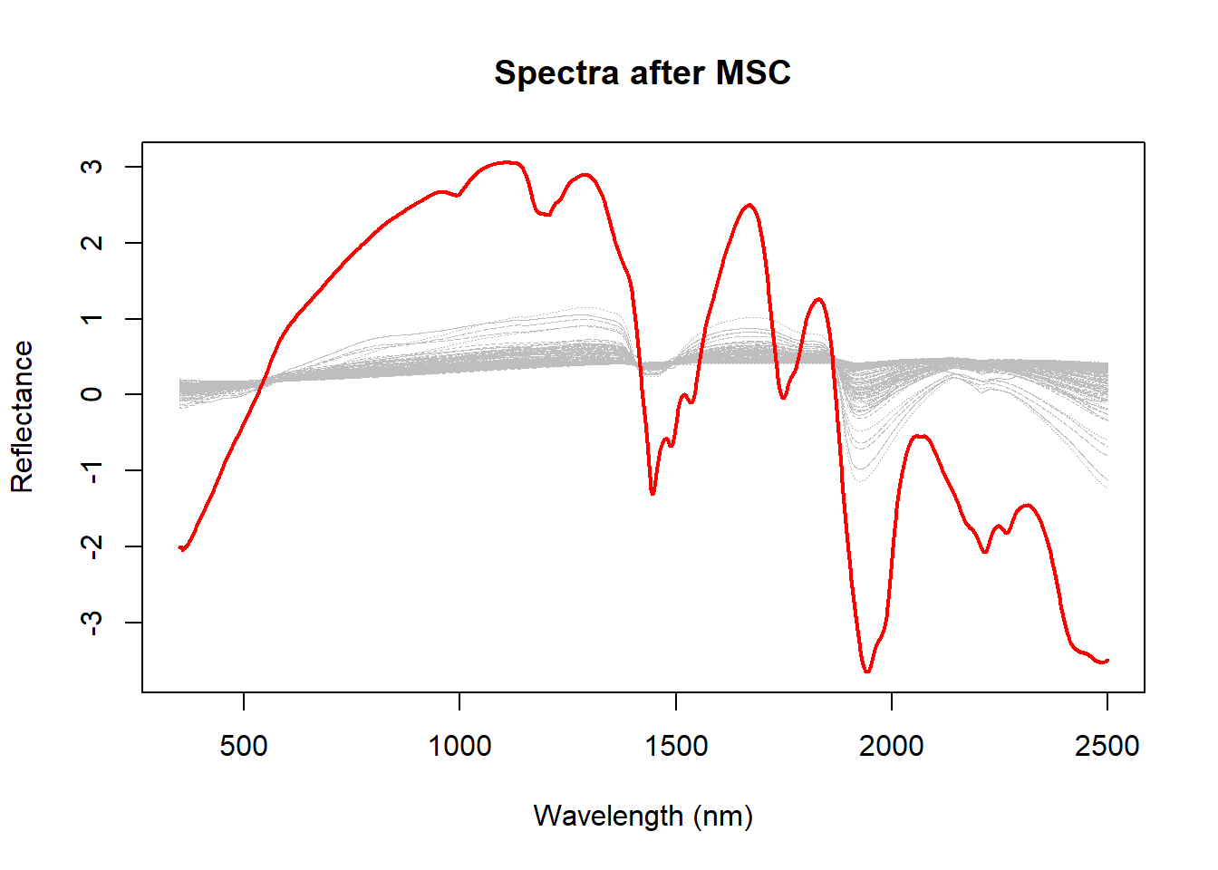
Remove this sample and calculate the MSC again:

msc_spectra <- msc(dat$spc[-msc_out_sample_index, ], ref_spectrum = colMeans(dat$spc[-msc_out_sample_index, ]))

matplot(colnames(dat$spc),
  t(msc_spectra),
  type = "l",
  col = "grey",
  lwd = 0.5,
  xlab = "Wavelength (nm)",
  ylab = "Reflectance",
  main = "Spectra after MSC"
)